UGC-NET COMPUTER SCIENCE PAPER-2 DECEMBER 2004 Answer Key with Explanation

Q::31. Which activity is not included in the first pass of two pass assemblers?

(A) Build the symbol table

(B) Construct the intermediate code

(C) Separate mnemonic opcode and operand fields

(D) None of the above

Answer: D

Explanation:

An assembler is a translator, that translates an assembler program into a conventional machine language program. Basically, the assembler goes through the program one line at a time, and generates machine code for that instruction. Then the assembler procedes to the next instruction. In this way, the entire machine code program is created. For most instructions this process works fine, for example for instructions that only reference registers, the assembler can compute the machine code easily, since the assembler knows where the registers are.

Consider an assembler instruction like the following

          JMP  LATER
          ...
          ...
LATER:

This is known as a forward reference. If the assembler is processing the file one line at a time, then it doesn't know where LATER is when it first encounters the jump instruction. So, it doesn't know if the jump is a short jump, a near jump or a far jump. There is a large difference amongst these instructions. They are 2, 3, and 5 bytes long respectively. The assembler would have to guess how far away the instruction is in order to generate the correct instruction. If the assembler guesses wrong, then the addresses for all other labels later in the program woulds be wrong, and the code would have to be regenerated. Or, the assembler could alway choose the worst case. But this would mean generating inefficiency in the program, since all jumps would be considered far jumps and would be 5 bytes long, where actually most jumps are short jumps, which are only 2 bytes long.

Soooooooo, what is to be done to allow the assembler to generate the correct instruction? Answer: scan the code twice. The first time, just count how long the machine code instructions will be, just to find out the addresses of all the labels. Also, create a table that has a list of all the addresses and where they will be in the program. This table is known as the symbol table. On the second scan, generate the machine code, and use the symbol table to determine how far away jump labels are, and to generate the most efficient instruction.

This is known as a two-pass assembler. Each pass scans the program, the first pass generates the symbol table and the second pass generates the machine code.

First Pass

On the first pass, the assembler performs the following tasks:

• Checks to see if the instructions are legal in the current assembly mode.
• Allocates space for instructions and storage areas you request.
• Fills in the values of constants, where possible.
• Builds a symbol table, also called a cross-reference table, and makes an entry in this table for every symbol it encounters in the label field of a statement.

The assembler reads one line of the source file at a time. If this source statement has a valid symbol in the label field, the assembler ensures that the symbol has not already been used as a label. If this is the first time the symbol has been used as a label, the assembler adds the label to the symbol table and assigns the value of the current location counter to the symbol. If the symbol has already been used as a label, the assembler returns the error message Redefinition of symbol and reassigns the symbol value.

Next, the assembler examines the instruction's mnemonic. If the mnemonic is for a machine instruction that is legal for the current assembly mode, the assembler determines the format of the instruction (for example, XO format). The assembler then allocates the number of bytes necessary to hold the machine code for the instruction. The contents of the location counter are incremented by this number of bytes.

When the assembler encounters a comment (preceded by a # (pound sign)) or an end-of-line character, the assembler starts scanning the next instruction statement. The assembler keeps scanning statements and building its symbol table until there are no more statements to read.

At the end of the first pass, all the necessary space has been allocated and each symbol defined in the program has been associated with a location counter value in the symbol table. When there are no more source statements to read, the second pass starts at the beginning of the program.

Note: If an error is found in the first pass, the assembly process terminates and does not continue to the second pass. If this occurs, the assembler listing only contains errors and warnings generated during the first pass of the assembler.

Second Pass

On the second pass, the assembler:

• Examines the operands for symbolic references to storage locations and resolves these symbolic references using information in the symbol table.
• Ensures that no instructions contain an invalid instruction form.
• Translates source statements into machine code and constants, thus filling the allocated space with object code.
• Produces a file containing error messages, if any have occurred.

At the beginning of the second pass, the assembler scans each source statement a second time. As the assembler translates each instruction, it increments the value contained in the location counter.

If a particular symbol appears in the source code, but is not found in the symbol table, then the symbol was never defined. That is, the assembler did not encounter the symbol in the label field of any of the statements scanned during the first pass, or the symbol was never the subject of a .comm, .csect, .lcomm, .sect, or .set pseudo-op.

This could be either a deliberate external reference or a programmer error, such as misspelling a symbol name. The assembler indicates an error. All external references must appear in a .extern or .globl statement.

The assembler logs errors such as incorrect data alignment. However, many alignment problems are indicated by statements that do not halt assembly. The -w flag must be used to display these warning messages.

After the programmer corrects assembly errors, the program is ready to be linked.

Note:

If only warnings are generated in the first pass, the assembly process continues to the second pass. The assembler listing contains errors and warnings generated during the second pass of the assembler. Any warnings generated in the first pass do not appear in the assembler listing.

Q::32. Which of the following is not collision resolution technique?

(A) Hash addressing (B) Chaining

(C) Both (A) and (B) (D) Indexing

Answer: D

Explanation:

Open addressing, or closed hashing, is a method of collision resolution in hash tables. With this method a hash collision is resolved by probing, or searching through alternate locations in the array (the probe sequence) until either the target record is found, or an unused array slot is found, which indicates that there is no such key in the table. Well known probe sequences include:

Linear probing  in which the interval between probes is fixed — often at 1.

Quadratic probing  in which the interval between probes increases linearly (hence, the indices are described by a quadratic function).

Double hashing in which the interval between probes is fixed for each record but is computed by another hash function.

Chaining

Hash collision resolved by separate chaining.

In the method known as separate chaining, each bucket is independent, and has some sort of list of entries with the same index. The time for hash table operations is the time to find the bucket (which is constant) plus the time for the list operation.
In a good hash table, each bucket has zero or one entries, and sometimes two or three, but rarely more than that. Therefore, structures that are efficient in time and space for these cases are preferred. Structures that are efficient for a fairly large number of entries per bucket are not needed or desirable. If these cases happen often, the hashing is not working well, and this needs to be fixed.

Indexing:
Indexing is a data structure technique to efficiently retrieve records from the database files based on some attributes on which the indexing has been done. Indexing in database systems is similar to what we see in books.
Indexing is defined based on its indexing attributes. Indexing can be of the following types −

Primary Index − Primary index is defined on an ordered data file. The data file is ordered on a key field. The key field is generally the primary key of the relation.


Secondary Index − Secondary index may be generated from a field which is a candidate key and has a unique value in every record, or a non-key with duplicate values.


Clustering Index − Clustering index is defined on an ordered data file. The data file is ordered on a non-key field.

Q::33. Code optimization is responsibility of: 

(A) Application programmer 

(B) System programmer 

(C) Operating system 

(D) All of the above 

Answer: B

Explanation:

Code optimization is any method of code modification to improve code quality and efficiency. A program may be optimized so that it becomes a smaller size, consumes less memory, executes more rapidly, or performs fewer input/output operations.

The basic requirements optimization methods should comply with, is that an optimized program must have the same output and side effects as its non-optimized version. This requirement, however, may be ignored in the case that the benefit from optimization, is estimated to be more important than probable consequences of a change in the program behavior.

In optimization, high-level general programming constructs are replaced by very efficient low-level programming codes. A code optimizing process must follow the three rules given below: 

The output code must not, in any way, change the meaning of the program. Optimization should increase the speed of the program and if possible, the program should demand less number of resources. 

Optimization should itself be fast and should not delay the overall compiling process.  Efforts for an optimized code can be made at various levels of compiling the process. At the beginning, users can change/rearrange the code or use better algorithms to write the code. After generating intermediate code, the compiler can modify the intermediate code by address calculations and improving loops. While producing the target machine code, the compiler can make use of memory hierarchy and CPU registers. 

Q::34 Which activity is included in the first pass of two pass assemblers?

(A) Build the symbol table

(B) Construct the intermediate code

(C) Separate mnemonic opcode and operand fields

(D) None of these

Answer: A,B,C

Explanation:

Refer to Question no. 31

Q::35.In two pass assembler the symbol table is used to store:

(A) Label and value    (B) Only value

(C) Mnemonic              (D) Memory Location

Answer: D

Refer to Question no. 31

Q::36.Semaphores are used to:

(A) Synchronise critical resources to prevent deadlock

(B) Synchronise critical resources to prevent contention

(C) Do I/o

(D) Facilitate memory management

Answer: 
Explanation:

A semaphore, in its most basic form, is a protected integer variable that can facilitate and restrict access to shared resources in a multi-processing environment. The two most common kinds of semaphores are counting semaphores and binary semaphores. Counting semaphores represent multiple resources, while binary semaphores, as the name implies, represents two possible states (generally 0 or 1; locked or unlocked). Semaphores were invented by the late Edsger Dijkstra.

Semaphores can be looked at as a representation of a limited number of resources, like seating capacity at a restaurant. If a restaurant has a capacity of 50 people and nobody is there, the semaphore would be initialized to 50. As each person arrives at the restaurant, they cause the seating capacity to decrease, so the semaphore in turn is decremented. When the maximum capacity is reached, the semaphore will be at zero, and nobody else will be able to enter the restaurant. Instead the hopeful restaurant goers must wait until someone is done with the resource, or in this analogy, done eating. When a patron leaves, the semaphore is incremented and the resource becomes available again.

A semaphore can only be accessed using the following operations: wait() and signal(). wait() is called when a process wants access to a resource. This would be equivalent to the arriving customer trying to get an open table. If there is an open table, or the semaphore is greater than zero, then he can take that resource and sit at the table. If there is no open table and the semaphore is zero, that process must wait until it becomes available. signal() is called when a process is done using a resource, or when the patron is finished with his meal. 

Page 1 2 3 4 5 6 7 8 9 10

ugc net computer science question papers,ugc net computer science december 2014 question papers,

ugc net computer science june 2014 question papers,

ugc net computer science december 2014 question papers,

ugc net computer science june 2013 question papers,

ugc net computer science december 2013 question papers,

ugc net computer science june 2012 question papers,

ugc net computer science december 2012 question papers,

ugc net computer science june 2011 question papers,

ugc net computer science december 2011 question papers,

ugc net computer science june 2010 question papers,

ugc net computer science december 2010 question papers,

ugc net computer science june 2009 question papers,

ugc net computer science december 2009 question papers,

ugc net computer science june 2008 question papers,

ugc net computer science december 2008 question papers,

december 2004 ugc net computer science paper,ugc net computer science december 2004 solution, cbse net all solved papers, cbse net 

UGC-NET COMPUTER SCIENCE DECEMBER 2004 Answer Key with Explanation

Q::26.Error control is needed at the transport layer because of potential error occurring ..............

(A) from transmission line noise

(B) in router

(C) from out of sequence delivery

(D) from packet losses

Answer:

Explanation:
TCP is a reliable transport layer protocol. This means that an application program that delivers a stream of data to TCP relies on TCP to deliver the entire stream to the application program on the other end in order, without error, and without any part lost or duplicated. TCP provides reliability using error control. Error control includes mechanisms for detecting corrupted segments, lost segments, out-of-order segments, and duplicated segments. Error control also includes a mechanism for correcting errors after they are detected. Error detection and correction in TCP is achieved through the use of three simple tools: checksum, acknowledgment, and time-out.

Q::27. Making sure that all the data packets of a message are delivered to the destination is ................ control.

(A) Error (B) Loss

(C) Sequence (D) Duplication

Answer: A


Q::28. Which transport class should be used with a perfect network layer?
(A) TP0 and TP2 (B) TP1 and TP3

(C) TP0, TP1, TP3 (D) TP0, TP1, TP2, TP3, TP4

Answer: A

Q::29. Which transport class should be used with residual-error network layer? 

(A) TP0, TP2 (B) TP1, TP3 

(C) TP1, TP3, TP4 (D) TP0, TP1, TP2, TP3, TP4 

Answer: B 

Q::30. Virtual circuit is associated with a ..................... service.



(A) Connectionless (B) Error-free



(C) Segmentation (D) Connection-oriented



Answer: D


Explanation:

A virtual-circuit network is a cross between a circuit-switched network and a datagram network. It 
has some characteristics of both.

(a)As in a circuit-switched network, there are setup and teardown phases in addition to the data transfer phase.

(b) Resources can be allocated during the setup phase, as in a circuit-switched network,

or on demand, as in a datagram network. 

(c) As in a datagram network, data are packetized and each packet carries an address in

the header. However, the address in the header has local jurisdiction (it defines what

should be the next switch and the channel on which the packet is being canied), not

end-to-end jurisdiction.

(d) As in a circuit-switched network, all packets follow the same path established during

the connection.

(e) A virtual-circuit network is normally implemented in the data link layer, while a

circuit-switched network is implemented in the physical layer and a datagram network

in the network layer. But this may change in the future.

Page 1 2 3 4 5 6 7 8 9 10

ugc net computer science question papers,ugc net computer science december 2014 question papers,

ugc net computer science june 2014 question papers,

ugc net computer science december 2014 question papers,

ugc net computer science june 2013 question papers,

ugc net computer science december 2013 question papers,

ugc net computer science june 2012 question papers,

ugc net computer science december 2012 question papers,

ugc net computer science june 2011 question papers,

ugc net computer science december 2011 question papers,

ugc net computer science june 2010 question papers,

ugc net computer science december 2010 question papers,

ugc net computer science june 2009 question papers,

ugc net computer science december 2009 question papers,

ugc net computer science june 2008 question papers,

ugc net computer science december 2008 question papers,

december 2004 ugc net computer science paper,ugc net computer science december 2004 solution, cbse net all solved papers, cbse net 

UGC-NET COMPUTER SCIENCE PAPER-2 DECEMBER 2004 Answer Key with Explanation

Q::21.       What item is at the root after the following sequence of insertions into an empty splay tree:

1, 11, 3, 10, 8, 4, 6, 5, 7, 9, 2 ?

(A) 1       (B) 2

(C) 4       (D) 8

Answer: B

Explanation:

A splay tree is a self-adjusting binary search tree with the additional property that recently accessed elements are quick to access again. It performs basic operations such as insertion, look-up and removal in O(log n) amortized time(amortized analysis is a method for analyzing a given algorithm's time complexity). For many sequences of non-random operations, splay trees perform better than other search trees, even when the specific pattern of the sequence is unknown. The splay tree was invented by Daniel Dominic Sleator and Robert Endre Tarjan in 1985.

All normal operations on a binary search tree are combined with one basic operation, called splaying. Splaying the tree for a certain element rearranges the tree so that the element is placed at the root of the tree. One way to do this is to first perform a standard binary tree search for the element in question, and then use tree rotations in a specific fashion to bring the element to the top. Alternatively, a top-down algorithm can combine the search and the tree reorganization into a single phase.

For more details visit 

http://cbsenetmaterial.blogspot.in/2015/11/ugc-net-computer-science-splay-tree.html

Q::22.       Suppose we are implementing quadratic probing with a Hash function, Hash (y)=X mode 100. If an element with key 4594 is inserted and the first three locations attempted are already occupied, then the next cell that will be tried is:

(A) 2       (B) 3

(C) 9       (D) 97

Answer: B

Explanation:

h(4594) = 94 i.e. our first attempt

94 + 1^2 = 95 second attempt

94 + 2^2 = 98 third attempt

94 + 3^2 = 103 % 100 = 3 i.e. next cell to be tried will be 3.

Q::23. Weighted graph:

(A) Is a bi-directional graph

(B) Is directed graph

(C) Is graph in which number associated with arc

(D) Eliminates table method

Answer: C

Explanation:
A weight is a numerical value, assigned as a label to a vertex or edge of a graph. A weighted graph is a graph whose vertices or edges have been assigned weights; more specifically, a vertex-weighted graph has weights on its vertices and an edge-weighted graph has weights on its edges. The weight of a subgraph is the sum of the weights of the vertices or edges within that subgraph.

Q::24. What operation is supported in constant time by the doubly linked list, but not by the singly linked list?

(A) Advance     (B) Backup

(C) First            (D) Retrieve

Answer: B

Q::25.       How much extra space is used by heap sort?

(A) O(1)              (B) O(Log n)

(C) O(n)             (D) O(n²)

Answer: A

Explanation:

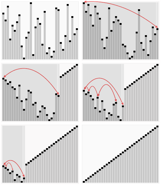
A run of the heapsort algorithm sorting an array of randomly permuted values. In the first stage of the algorithm the array elements are reordered to satisfy the heap property. Before the actual sorting takes place, the heap tree structure is shown briefly for illustration.
Class	Sorting algorithm
Data structure	Array
Worst case performance
Best case performance	[1]
Average case performance
Worst case space complexity	auxiliary

Page 1 2 3 4 5 6 7 8 9 10

ugc net computer science question papers,ugc net computer science december 2014 question papers,

ugc net computer science june 2014 question papers,

ugc net computer science december 2014 question papers,

ugc net computer science june 2013 question papers,

ugc net computer science december 2013 question papers,

ugc net computer science june 2012 question papers,

ugc net computer science december 2012 question papers,

ugc net computer science june 2011 question papers,

ugc net computer science december 2011 question papers,

ugc net computer science june 2010 question papers,

ugc net computer science december 2010 question papers,

ugc net computer science june 2009 question papers,

ugc net computer science december 2009 question papers,

ugc net computer science june 2008 question papers,

ugc net computer science december 2008 question papers,

december 2004 ugc net computer science paper,ugc net computer science december 2004 solution, cbse net all solved papers, cbse net 

UGC-NET Computer Science December 2004 Answer Key with Explanation

Q::16. The E-R model is expressed in terms of:

(i) Entities

(ii) The relationship among entities

(iii) The attributes of the entities

Then

(A) (i) and (iii)

(B) (i), (ii) and (iii)

(C) (ii) and (iii)

(D) None of the above
Answer: B

Explanation:
      The entity-relationship (E-R) data model perceives the real world as consisting of basic objects, called entities, and relationships among these objects. It was developed to facilitate database design by allowing specification of an enterprise schema, which represents the overall logical structure of a database. The E-R data model is one of several semantic data models; the semantic aspect of the model lies in its representation of the meaning of the data. The E-R model is very useful in mapping the meanings and interactions of real-world enterprises onto a conceptual schema. Because of this usefulness, many database-design tools draw on concepts from the E-R model.

Q::17. Specialization is a ............... process.

(A) Top - down (B) Bottom -Up

(C) Both (A) and (B) (D) None of the above

Answer: A

Explanation:

The process of designating subgroupings within an entity set is called specialization.An entity set may include subgroupings of entities that are distinct in some way from other entities in the set. For instance, a subset of entities within an entity set may have attributes that are not shared by all the entities in the entity set. The E-R model provides a means for representing these distinctive entity groupings. Consider an entity set person, with attributes name, street, and city. 

A person may be further classified as one of the following:

• customer

• employee

Each of these person types is described by a set of attributes that includes all the attributes of entity set person plus possibly additional attributes. For example, customer entities may be described further by the attribute customer-id, whereas employee entities may be described further by the attributes employee-id and salary.The specialization of person allows us to distinguish among persons according to whether they are employees or customers.

Q::18.    The completeness constraint has rules:

   (A) Supertype, Subtype

   (B) Total specialization, Partial specialization

   (C) Specialization, Generalization

   (D) All of the above

Answer: B

Explanation:

The completeness constraint on a generalization or specialization, specifies whether or not an entity in the higher-level entity set must belong to at least one of the lower-level entity sets within the generalization/specialization. This constraint may be one of the following:

• Total generalization or specialization:Each higher-level entity must belong to a lower-level entity set.

• Partial generalization or specialization: Some higher-level entities may not belong to any lower-level entity set.

Partial generalization is the default.We can specify total generalization in an E-R diagram by using a double line to connect the box representing the higher-level entity set to the triangle symbol.

We can see that certain insertion and deletion requirements follow from the constraints that apply to a given generalization or specialization. For instance, when a total completeness constraint is in place, an entity inserted into a higher-level entity set must also be inserted into at least one of the lower-level entity sets. With a condition-defined constraint, all higher-level entities that satisfy the condition must be inserted into that lower-level entity set. Finally, an entity that is deleted from a higher-level entity set also is deleted from all the associated lower-level entity sets to which it belongs.

Q::19.   The entity type on which the ................. type depends is called the identifying owner.

   (A) Strong entity                  (B) Relationship

   (C) Weak entity                     (D) E - R

Answer: C

Explanation:
An entity set may not have sufficient attributes to form a primary key. Such an entity set is termed a weak entity set. An entity set that has a primary key is termed a strong entity set. As an illustration, consider the entity set payment, which has the three attributes: {payment-number, payment-date, payment-amount}. Payment numbers are typically sequential numbers, starting from 1, generated separately for each loan. Thus, although each payment entity is distinct, payments for different loans may share the same payment number. Thus, this entity set does not have a primary key; it is a weak

entity set. For a weak entity set to be meaningful, it must be associated with another entity set, called the identifying or owner entity set. Every weak entity must be associated with an identifying entity; that is, the weak entity set is said to be existence dependent on the identifying entity set. The identifying entity set is said to own the weak entity set that it identifies. The relationship associating the weak entity set with the identifying entity set is called the identifying relationship. The identifying relationship is many to one from the weak entity set to the identifying entity set, and the participation of the weak entity set in the relationship is total. In our example, the identifying entity set for payment is loan, and a relationship loan-payment that associates payment entities with their corresponding loan entities is the identifying relationship. Although a weak entity set does not have a primary key, we nevertheless need a means of distinguishing among all those entities in the weak entity set that depend on one particular strong entity. The discriminator of a weak entity set is a set of attributes that allows this distinction to be made. For example, the discriminator of the weak entity set payment is the attribute payment-number, since, for each loan, a payment number uniquely identifies one single payment for that loan. The discriminator of a weak entity set is also called the partial key of the entity set. The primary key of a weak entity set is formed by the primary key of the identifying entity set, plus the weak entity set’s discriminator. In the case of the entity set payment, its primary key is {loan-number, payment-number}, where loan-number is the primary key of the identifying entity set, namely loan, and payment-number distinguishes payment entities within the same loan.

Q::20.    Match the following:

(i) 5 NF              (a) Transitive dependencies eliminated

(ii) 2 NF             (b) Multivalued attribute removed

(iii) 3 NF             (c) Contains no partial functional dependencies

(iv) 4 NF             (d) Contains no join dependency

(A) i-a, ii-c, iii-b, iv-d    

(B) i-d, ii-c, iii-a, iv-b

(C) i-d, ii-c, iii-b, iv-a   

(D) i-a, ii-b, iii-c, iv-d

Answer: B

Explanation:
First Normal Form

The first of the normal forms that we study, first normal form, imposes a very basic requirement on relations; unlike the other normal forms, it does not require additional information such as functional dependencies. A domain is atomic if elements of the domain are considered to be indivisible units. We say that a relation schema R is in first normal form (1NF) if the domains of all attributes of R are atomic. A set of names is an example of a nonatomic value. For example, if the schema of a relation employee included an attribute children whose domain elements are sets of names, the schema would not be in first normal form. Composite attributes, such as an attribute address with component attributes street and city, also have non-atomic domains.

Second Normal Form

A table that is in first normal form (1NF) must meet additional criteria if it is to qualify for second normal form. Specifically: a table is in 2NF if it is in 1NF and no non-prime attribute is dependent on any proper subset of any candidate key of the table. A non-prime attribute of a table is an attribute that is not a part of any candidate key of the table.A functional dependency on part of any candidate key is a violation of 2NF. In addition to the primary key, the table may contain other candidate keys; it is necessary to establish that no non-prime attributes have part-key dependencies on any of these candidate keys.

Third Normal Form

A relation schema R is in third normal form (3NF) with respect to a set F of functional

dependencies if, for all functional dependencies in F+ of the form α → β,

where α ⊆ R and β ⊆ R, at least one of the following holds:

• α → β is a trivial functional dependency.

• α is a superkey for R.

• Each attribute A in β − α is contained in a candidate key for R.

Note that the third condition above does not say that a single candidate key should

contain all the attributes in β − α; each attribute A in β − α may be contained in a

different candidate key.

The first two alternatives are the same as the two alternatives in the definition of

BCNF. The third alternative of the 3NF definition seems rather unintuitive, and it is

not obvious why it is useful. It represents, in some sense, a minimal relaxation of the

BCNF conditions that helps ensure that every schema has a dependency-preserving

decomposition into 3NF. Any schema that satisfies BCNF also satisfies 3NF, since each of its

functional dependencies would satisfy one of the first two alternatives. BCNF is therefore

a more restrictive constraint than is 3NF.

The definition of 3NF allows certain functional dependencies that are not allowed

in BCNF. A dependency α → β that satisfies only the third alternative of the 3NF

definition is not allowed in BCNF, but is allowed in 3NF.

For more please refer to Silberschatz−Korth−Sudarshan:Database System Concepts.

Page 1 2 3 4 5 6 7 8 9 10

ugc net computer science question papers,ugc net computer science december 2014 question papers,

ugc net computer science june 2014 question papers,

ugc net computer science december 2014 question papers,

ugc net computer science june 2013 question papers,

ugc net computer science december 2013 question papers,

ugc net computer science june 2012 question papers,

ugc net computer science december 2012 question papers,

ugc net computer science june 2011 question papers,

ugc net computer science december 2011 question papers,

ugc net computer science june 2010 question papers,

ugc net computer science december 2010 question papers,

ugc net computer science june 2009 question papers,

ugc net computer science december 2009 question papers,

ugc net computer science june 2008 question papers,

ugc net computer science december 2008 question papers,

december 2004 ugc net computer science paper,ugc net computer science december 2004 solution, cbse net all solved papers, cbse net june 2015 paper 2 solution computer science,